1 Data Clean Up
Task explanation.
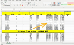
Set yourself in a situation where you own a bunch of used car dealerships all around canada and you are given a report of the sales. The sales report looks nice but has many limitations. You are looking for totals and would like to sort by Sales person and by Brand but all this doesn't seem possible. Changing numbers don't change the totals and many factors seem out of place.
All this makes you uneasy to say the least. You recently took an excel class that showed you what data practices you would have to follow to be able to look into those numbers better.
Could you clean up this dataset so that it can be used for further analysis?

🌶 Spicy Challenge. 🌶

How to details.
Alright so there is a bunch of things wrong with this file that needs to be removed so that Excel can start computing the numbers behind it.
First thing is to make sure your data starts in A1 and doesn't countain 2 rows of Titles. Let's right click on the Row 1 filed with merge cells and hit delete. You could choose to add shapes to maintain this information.
If you want to add shapes to your excel file you need to go under the Insert TAB, in the Illustrations chunk to select the shapes you would want!

Now the titles are cleaned up, we have some more work to do when it comes to the Provincial separators. We have lines in the data that hold totals and the information related to provinces for each of this data.
This is wrong evidently because of the merge cells but also it is a bad practice to divide your data with separators. You could easily just hit Delete on each row to get rid of them. The problem is that you might lose the information related to the provinces. Since there is no Collumn called Province you will need to add one and fill the info in all that collumn.
First type the name of the province and use the FILL Cursor to populate the data in that collumn. Once it's populated, remove the separator. Do this over and over until your province collumn is full and the all the separators are removed

Once this is done you are really close to success, your dataset has no merges anymore you removed the separators and kept the provincial information in a new collumn.
Another malpractice in this data is the B,C,D collumns which represent Type of vehible. Ideally, this information would be located only in 1 collumn called TYPE. The issue here will require combining the 3 collumns. One easy way to fix this is to sort the collumns D, C and then B and once they are in order it will be easy for you to once again use the Fill cursor to populate the data in those collumns.
To do this Right click the first cells of each collumn and choose to sort them from A to Z. After that Type in the name and fill it down. Once it's all done, delete your 3 collumns and only keep the first one.

Finally, after all this is clean and done. You are missing one last collumn to make sure all this works wonderful.
The ID Collumn. Select Collumn A and insert a new collumn. Call it ID and type 1 in A2 and 2 in A3 and then double click the fill cursor when selecting both.
Now you have a proper range of data ready for tables and pivot tables. This is also valid for exporting to online data or to databases


