6 Shipping Prices
Task explanation.
We gave free shipping on a bunch of invoices. 2713 to be clear. We are trying to figure out what is the amount of money we paid for shipping.
Download the document and check the shipping calculation table to calculate the total cost of our shipping policy last year.

🌶 Spicy Challenge. 🌶
Although this exercise is doable with better performance in 4 collumns. Would you be able to make all these functions fit into 1 massive 4 lookup nested function?

How to details.
Now this is one hell of an intimidating exercise if you attempt to do it with IF statements. Trying to figure out with IF would be a huge challenge, but it would be possible. The function would be long and very difficult to understand but it could be done.
Logically, if something like this would happen to you it would be way better to go on the path of LOOKUP functions since they let you find information located in a table.
This exercise has 4 tables to help find the end price.
We will build once again all the formulas one after the other and at the end I'll share the method to combine all of them into one. Note that for this particular exercise it's better for performance to keep them all separated.
So first we will use some simple APPROXIMATIVE VLOOKUPS to find their size and weight category.
Since VLOOKUP requires your data to be in numerical format and ascending this is what your tables needs to look like :

Now that your tables were modified to fit the requirements of Vlookup - You can now go ahead and jump into making it work!
STEP 1 of every VLOOKUP is to:
NAME THE RANGES
While you are at it you can create all the required names for this exercise.
THIS IS A CRITICAL STEP AND SKIPPING IT WILL MAKE EVERYTHING IN THIS EXERCISE FAIL
Here's the names I'll use
WeightTypeTable - B19 to C21
SizeTypeTable - B14 to C16
CatIndexTable - B9 to D11
CatMatchRows - A9 to A11
CatMatchColls - B8 to D8
PriceIndexTable - B3 to F5
PriceMatchRows - A3 to A5
PriceMatchColls - B2 to F2
And here is how you name the whole thing!
Select the range you want and go in the top left and type the name of the table and hit ENTER! Here's a gif to help you out :

That might of taken time but will end up being invaluable in the creation of the next functions since it will make it quick for us to build the other functions without going back to the SHIPPING CALCULATION TABLE sheet.
So let's get started with the functions :
First the functions for weight types is:
=VLOOKUP(B2,WeightTypeTable,2)
Second the function for size types is:
=VLOOKUP(C2,SizeTypeTable,2)
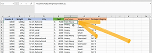
If you take the time to input these formulas inside F2 and G2 you should be able to have 2 collumns now that are able to define the Size and the Weight Types

Awesome!
Now that you have this information it will be possible to find the package category.
For this one you will require a INDEX/MATCH since the table requires information to be found from the top collumns and left rows.
We need to run 3 functions nested into each other
INDEX to find the info from the apt row and apt collumn
MATCH to find the Apt Row
MATCH to find the Apt Collumn
Here's what it would look like:
=INDEX(CatIndexTable,MATCH(G2,CatMatchRows,0),MATCH(F2,CatMatchColls,0))
Notice how we used all the previous names

Awesome... we are getting so close to our price. Now that we have the package categorie and the location information. We can finally produce our Cost finding function.
Again it's an INDEX/MATCH functions:
=INDEX(PriceIndexTable,MATCH(D2,PriceMatchRows,0),MATCH(H2,PriceMatchColls,0))
Here's how it looks in Excel

HURRAY! IT'S DONE WE FOUND ALL THE PRICES. Excel is amazing.
For The spicy Challenge
This last step isn't required because leaving this functions seperatly will reduce the workload of your document but if you want to see how you can combine this whole thing together into one crazy 4 lookup function here's a little gif to show you:


